Exploring Topographic Data with Transitive Closure on Graphs

This project brings database-style recursive query evaluation to plain Python/Pandas, and uses terrain as both a motivating application and a tunable benchmark. It will be presented at DEXA 2026 in Austria. This is joint work with Christoph F. Eick and Carlos Ordonez at the University of Houston.

The idea

Transitive closure — computing every reachable source/destination pair in a graph — is a foundational recursive query that is traditionally confined to database systems. This work shows that database-style fixpoint semantics can be implemented effectively and correctly in Pandas, making it practical for moderate-scale exploratory analysis without standing up a full database. Digital Elevation Models (DEMs) provide an ideal domain: they are large, structured, and produce graphs whose density can be tuned.

From terrain to graph

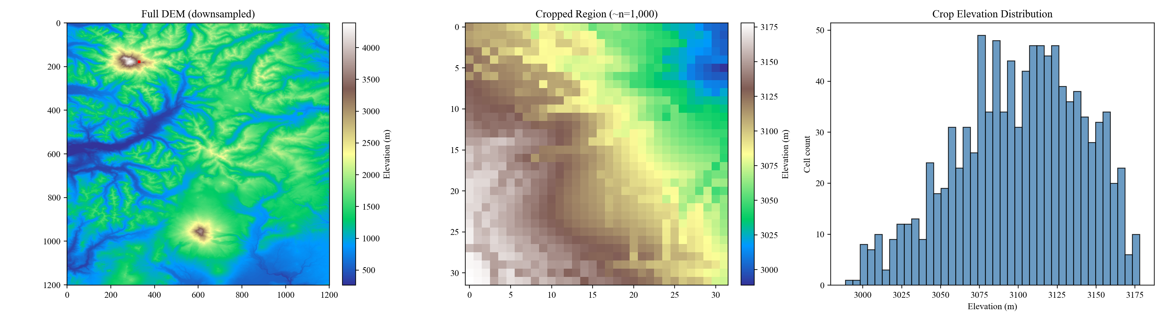
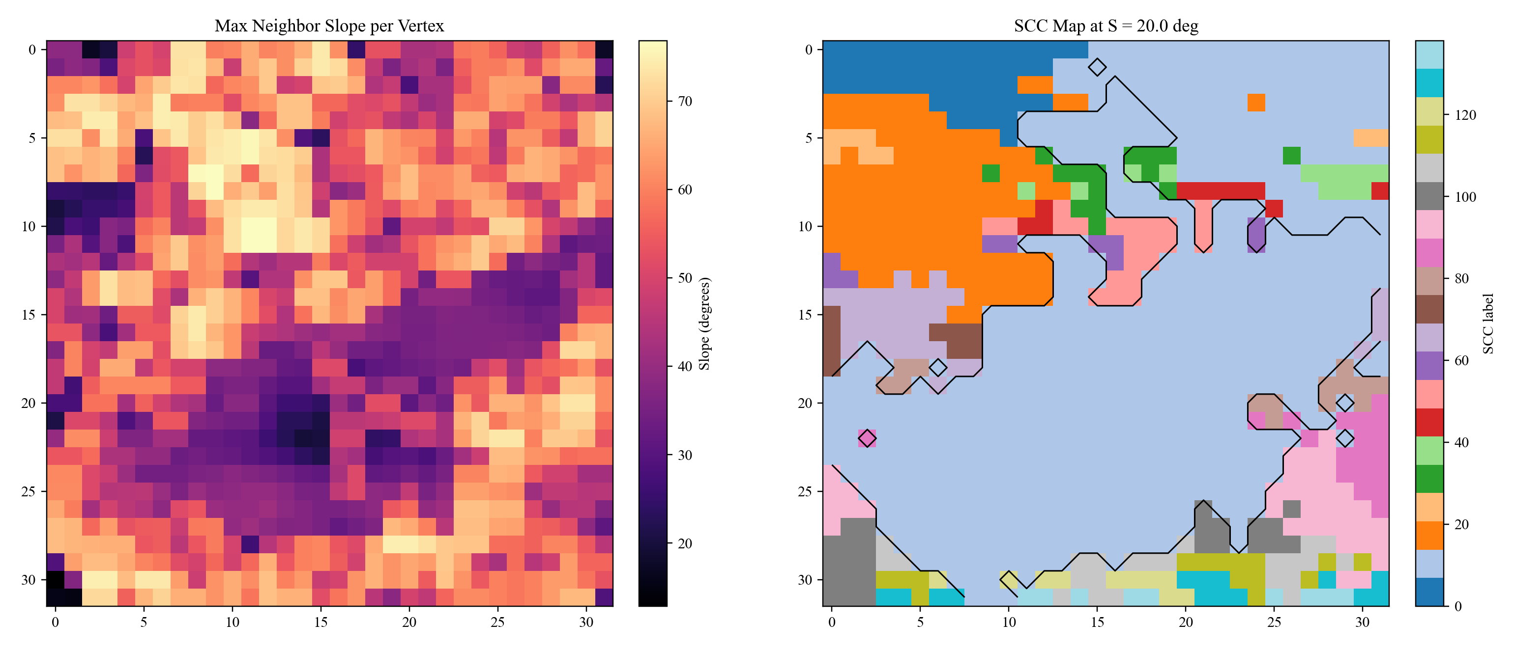
Full Mount Rainier DEM, the 32x32 cropped experiment region, and its elevation distribution — The USGS 3DEP source DEM (Mount Rainier), the 32×32 summit crop used for the n=1,000 experiments, and its elevation distribution.

A DEM is modeled as a directed graph: each cell is a vertex, and edges connect adjacent cells (8-connectivity). Each edge carries the signed elevation difference and the slope angle between the two cells.
A slope-passability threshold S filters which transitions are traversable. Crucially, S is treated as a query-time parameter — so a single physical terrain yields a whole family of graphs of varying density, without rewriting the underlying structure.
The graph construction is validated for structural invariants (antisymmetry, no self-loops, correct per-vertex degree, exact trigonometric slopes) and is O(n), scaling linearly to 1.6 billion cells.

Maximum neighbor slope per vertex beside the strongly connected components map at S=20 degrees — Left: maximum neighbor slope per vertex, showing the rugged topography. Right: strongly connected components at S = 20° — disparate regions become mutually reachable.

Computing the closure

The closure is computed with a seminaïve fixpoint over the slope-filtered edge set, which avoids redundantly recomputing known paths:

Require: Edge relation E(src, dst)
1:  TC ← E
2:  Δ  ← E
3:  while Δ ≠ ∅ do
4:      New ← Δ ⋈ E          // join the new frontier with base edges
5:      New ← New \ TC        // keep only newly discovered pairs
6:      TC  ← TC ∪ New
7:      Δ   ← New
8:  end while
9:  return TC

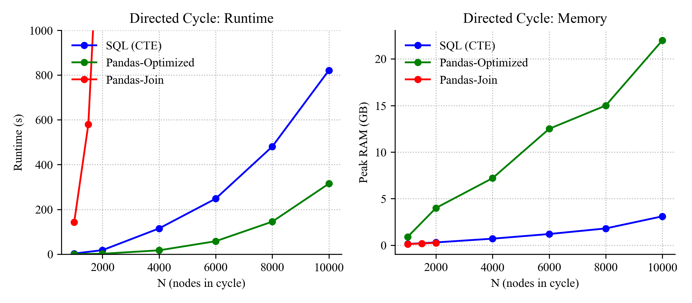
Correctness is checked against a SQLite recursive view used as an oracle: zero row discrepancy at every tested slope threshold. The seminaïve strategy runs 1.5–3.3× faster than naïve evaluation.

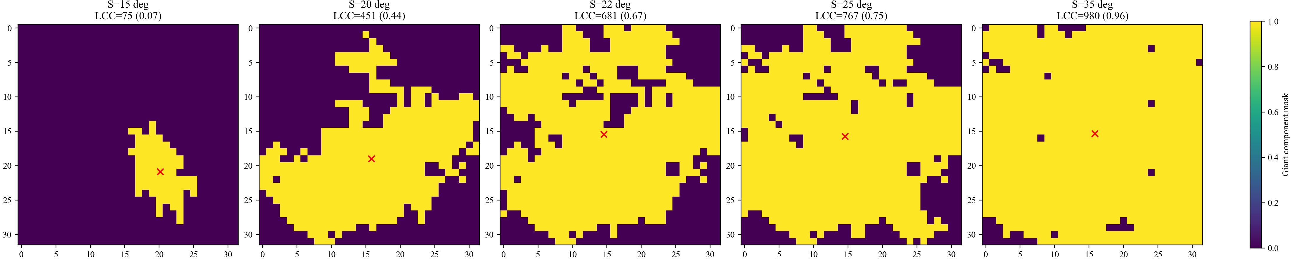
Runtime and peak memory versus cycle size for SQL CTE, optimized Pandas, and join-based Pandas — Directed-cycle stress test: the optimized Pandas engine beats the SQL CTE baseline on runtime, trading higher peak memory; a naïve join-based approach explodes almost immediately.

What the terrain reveals

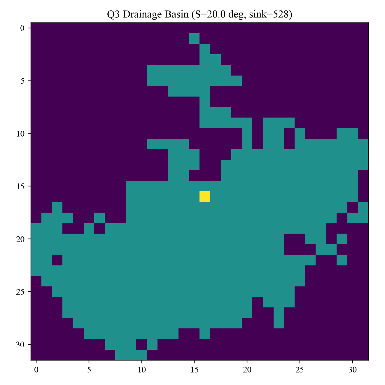
Sweeping the slope threshold S exposes a sharp structural phase transition near 20°: below it, the terrain fragments into hundreds of isolated components; above it, a giant mutually-reachable component dominates the map. That makes the terrain graph an excellent, controllable workload generator for recursive-query research.

Giant component masks at slope thresholds from 15 to 35 degrees, growing from 7 percent to 96 percent coverage — The giant component while sweeping S from 15° to 35°: coverage jumps from 7% of the terrain to 96%, with most of the change concentrated around the ~20° transition.

Once the closure is materialized as a DataFrame, ordinary Pandas operations answer rich topographic questions — turning relational lookups into geographic insight:

Point-to-point reachability — can you get from a trailhead to a summit within a slope tolerance?
Drainage basins — reverse-reachability into a valley outlet (useful for hydrological modeling).
Reachable hubs — the most central, flat gathering point from a location (e.g. a helicopter landing zone in search-and-rescue).
Bottleneck / choke-point detection — narrow land bridges whose removal would sever a route.
Shortest path — distance-aware traversal cost across slope-constrained terrain.

Drainage basin query output: cells draining into a highlighted sink at S=20 degrees — A drainage-basin query at S = 20°: one reverse-reachability lookup over the materialized closure paints every cell (teal) that drains into the highlighted sink.

Closure experiments run at n = 1,000 and n = 10,000 cells, with the construction step demonstrated to scale linearly well beyond that.